Profiling
Apple Mail MCP ships a --profile PATH flag on index and rebuild so
you can capture a performance trace of the indexing pipeline and share
it in a bug report — or use it locally to diagnose slow syncs on your
own mailbox.
The flag uses Python's stdlib cProfile, so there are no extra runtime
dependencies. Profile dumps are standard pstats-format files readable
by any Python profiling tool.
When to profile
- You're seeing slow
apple-mail-mcp indexorrebuildruns and want to know which layer is the bottleneck (disk walk vs.emlxparse vs HTML stripping vs SQLite inserts vs FTS5 rebuild). - You're filing a perf-related issue and want to give maintainers actionable data instead of just "this is slow on a 100k mailbox."
- You're evaluating a code change for its real cost on your own workload, not against the project's benchmarks (which run on a smaller fixture).
If you just want to know whether the index is healthy — not how fast
it builds — use apple-mail-mcp status instead.
Capture a profile
This runs the full disk-based index build wrapped in cProfile. The
.prof file is binary; it's a few MB even for a 100k+ mailbox.
The same flag works on rebuild:
The flag adds measurable overhead (typically 5-10% of wall-clock for the indexing operation), so don't leave it on for normal use.
Inspect the profile
Quick text summary
The simplest readout — sorted by where time was actually spent (self-time, excluding callees):
python -c "
import pstats
p = pstats.Stats('/tmp/sync.prof')
p.sort_stats('tottime').print_stats(20)
"
For "where does time flow through the call stack" (cumulative time, including callees):
python -c "
import pstats
p = pstats.Stats('/tmp/sync.prof')
p.sort_stats('cumulative').print_stats(25)
"
Flame chart (visual)
flameprof renders a
self-contained SVG that shows the full call-stack hierarchy with
box width proportional to time:
uv tool install flameprof   # one-time install
flameprof /tmp/sync.prof --width 1600 > /tmp/sync_flame.svg
open /tmp/sync_flame.svg
The flame chart has two halves stacked together:
- Top half (orange/yellow): cumulative time. Each box's width = total time spent in that function and everything it called. Vertical position = call stack depth (bottom = entry point, up = deeper in the stack). Read this to answer where in the codebase does work flow.
- Bottom half (grayscale): self time. Same call stack ordering, but width = time spent inside that function only, excluding callees. Wide bars here are the actual workers; narrow bars are scaffolding that just dispatches to children. Read this to answer which function should I optimize.
Call graph (alternative)
gprof2dot renders a directed
graph where nodes are functions, edges are calls, and edge thickness is
time:
uv tool install gprof2dot
brew install graphviz   # for the `dot` renderer
python -m gprof2dot -f pstats /tmp/sync.prof --node-thres=1.0 \
    | dot -Tsvg -o /tmp/sync_callgraph.svg
open /tmp/sync_callgraph.svg
Better for "how is the codebase structured under load" than "where is time going" — for the latter, prefer the flame chart.
Interactive exploration (local only)
snakeviz opens an interactive
sunburst in your browser:
Best for ad-hoc drill-down on your own machine; not useful for attaching to bug reports because it's not a static asset.
Sharing a profile in a bug report
The .prof file is small (a few MB even for large indexes) and
contains only function names, file paths from your installed Python
environment, and timing data. It does not contain message
content, email addresses, or filenames from your mailbox — only
references to internal Python functions like email.parser.parse or
apple_mail_mcp.index.disk.parse_emlx.
That said, the file paths in the dump do include your username
(e.g. /Users/<you>/Library/Mail/V10/... won't appear, but
/Users/<you>/.local/share/uv/python/... will). Strip your
username with sed before attaching if you'd rather not share it:
Then attach to the issue with a short note: mailbox size, machine
specs, wall-clock time, and the pstats text summary inline so
maintainers can read it without downloading the binary.
Reading a profile: what to look for
The right question to ask is which optimizations would change the breakdown, not just what is the largest line. Some patterns:
- One function dominates self-time (>40%): the optimization target is clear — that function is the bottleneck. Look for ways to call it less often or replace its implementation.
- No single function dominates; time is balanced across many small workers: this is the "death by a thousand cuts" pattern. Per-line optimizations won't help much; the right move is structural — do less work, not do work faster. Skip a phase entirely, cache an expensive computation, or use a different algorithm.
- A wide cumulative bar with thin self-time inside it: a router function. Optimizing it directly buys nothing; push down into its children.
- Time invariant with input size: classic sign of unconditional work. If a sync with 1 changed message takes the same wall-clock as a sync with 1000 changed messages, the work is happening independent of the diff result. Look for code paths that run regardless of state (often: full re-walks, full re-parses).
What this project knows so far
A reference profile of apple-mail-mcp index on a real ~60k-message
mailbox (M1 Pro, internal SSD, macOS 26.4):
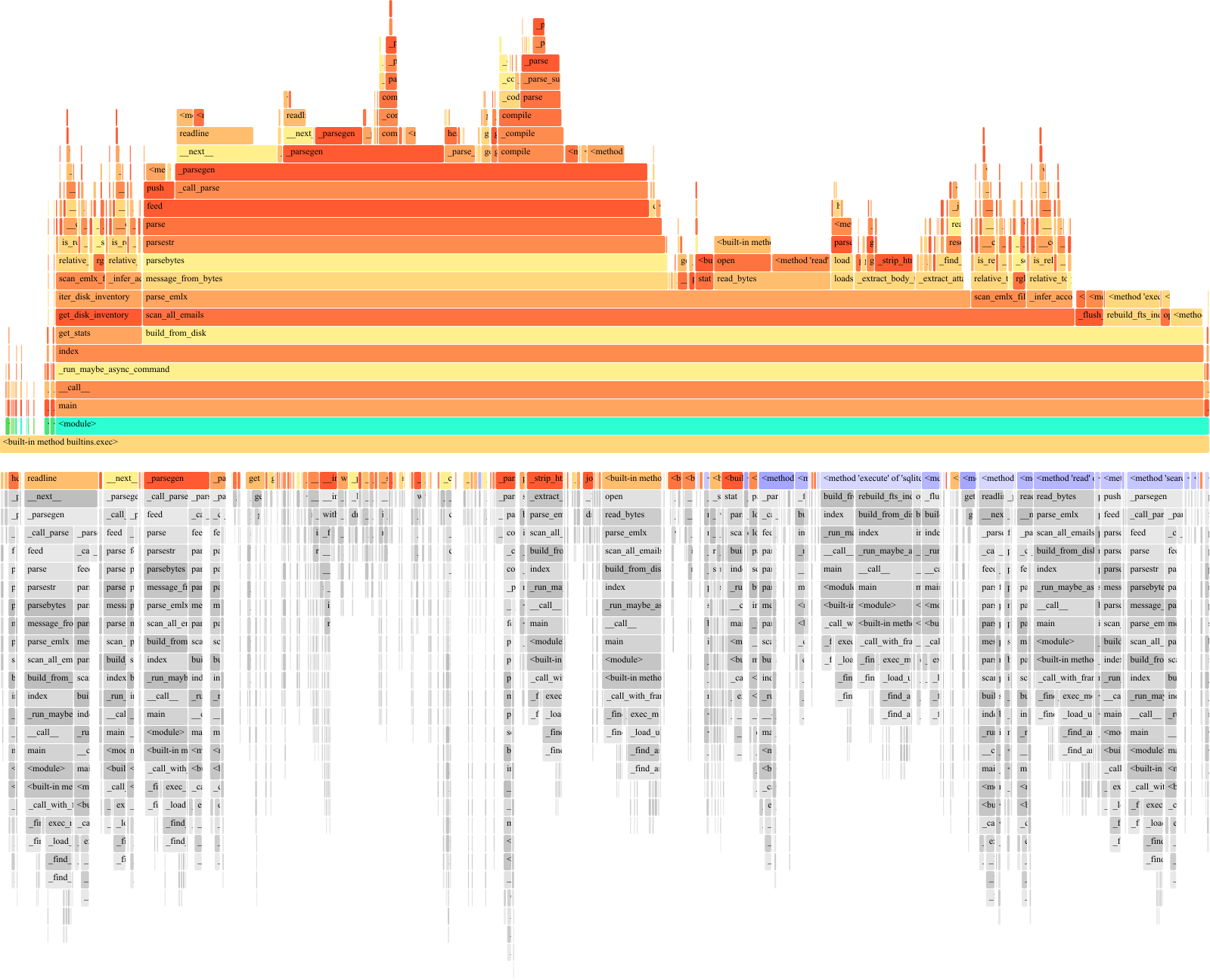
The chart's two halves answer different questions (top: cumulative time through the call stack; bottom: self-time spent inside each function). See "Flame chart (visual)" above for how to read each.
Aggregated by component:
| Component | Approximate share of self-time |
|---|---|
Stdlib email.parser internals |
~20% |
File I/O (open, read) |
~11% |
SQLite execute calls |
~8% |
| Regex matching | ~7% |
pathlib operations |
~5% |
HTML stripping (_strip_html) |
~3% |
| Other Python overhead | ~46% |
There is no single dominant bottleneck on this dataset. The disk walk
itself (scan_emlx_files) is only ~10% of cumulative time — most of
the cost is in parsing what the walk surfaces, not in the walk.
Larger mailboxes (200k+) and attachment-heavy archives may show different breakdowns. Profile your own data before assuming the above generalizes.